Introduction

I have just hit the merge button on the 0.4.1 release of JutulDarcy. There is a lot of nice improvements in the 0.4.0 and 0.4.1 releases, but the biggest change since the 0.3 series is full support for executing models on GPUs. We already had GPU support for linear solves on CUDA through NVIDIAs CuSPARSE and AMGX libraries, but the new release moves all compute-intensive parts to the GPUs in a single unified implementation that can execute on AMD GPUs, CUDA GPUs, OpenCL and different flavors of CPUs, all written in Julia.

Example of a 300 by 300 mesh eeight-pseudocomponent Safah fluid from Hearn and Whitson, SPE 29115 in a quarter-five-spot displacement running on the GPU.

This post is written for those who are interested in at least one of the following:

• GPUs for reservoir simulation
• The Julia programming language
• Vendor neutral GPU programming
• AI assistance

This post is intended to be read by readers who may not be familiar with all of the above, so please bear with me if you are already a GPU-reservoir simulation expert who writes Julia kernels in your sleep (if so, drop me a line, we probably have some overlapping interests!).

I don’t want to read, I want numbers

Ok, then! Reported numbers are for a double precision solve with linear algebra in single precision and FGMRES as the outer solver.

SPE10

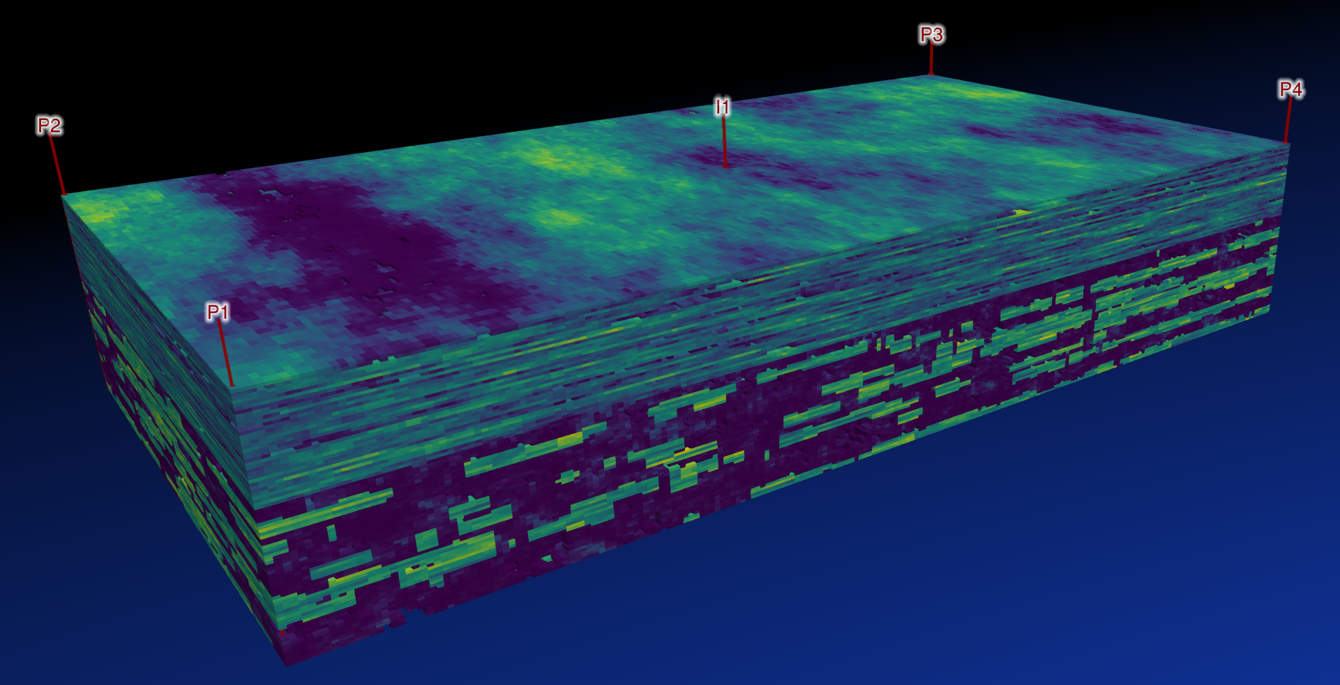
SPE10 (193 Newtons) in 12 seconds on a GTX 4080. On a Blackwell card this drops to under 8 seconds, with a single evaluation of properties and assembly taking less than 2 ms for the entire model.

SPE11

Solving a 2 million cell thermal SPE11b case uses 110 ms per complete iteration, where each property and assembly pass is less than 25 ms.

Hydrogen storage

The 8 component Underground Hydrogen Benchmark study (316 steps, 600 Newtons) runs in 50 seconds with the flash running on GPU. Here is a video in JutulDarcy’s viewer:

Real-field models

I cannot share too much about confidential models, but one example is a black-oil model with approximately 100 wells and 200,000 cells with 20 years of history that now runs in 70 seconds over 8 minutes on CPU. So even moderately sized models with a lot of smaller time-steps get improved performance.

JutulDarcy - Reservoir simulation in Julia

JutulDarcy is a toolkit for loading, visualizing, modifying, building, simulating and optimizing reservoir simulation models. It is used extensively in our research, and we release it as open source under a permissive license.

I started what eventually became Jutul.jl (automatic differentiation-based nonlinear solvers for discretized PDEs) and JutulDarcy.jl (reservoir simulation with Jutul.jl as the engine) back in 2020 with three goals:

1. Learn Julia well enough to confidently use it in ongoing projects at SINTEF (a success! I now use Julia a lot, as do many of my colleagues.)
2. Explore the potential for fast automatic differentiation of PDEs using the many AD packages in the Julia ecosystem¹ (definitely a success, even if we had to write a lot of code to get there)
3. Assess the potential for “write once, execute everywhere” GPU/CPU parallelism that was emerging through the then nascent KernelAbstractions package² (…it took six years, but we got there in the end…)

The initial version of the code contained AD solves for single and multiphase immiscible flow without any wells running on both CPU and GPU. Back in 2020, writing and testing kernels required a working GPU device, and the developer experience for kernel programming was very rough around the edges, with incomprehensible error messages and frequent crashes when launching kernels that gave errors. I made the decision to instead focus on differentiablity and high performance on the CPU. In the main paper “JutulDarcy.jl - a fully differentiable high-performance reservoir simulator based on automatic differentiation”, the GPU results are limited to the linear solvers for NVIDIA devices via CuSPARSE/AMGX vendor libraries. These do give noticable performance benefits, but having only the linear solver on GPU means that there is a lot of memory traffic between the device and host during each solve.

Overview of this blog post

This blog post is not about the great performance offered by GPUs, which is well established in the literature, but rather how reservoir simulation can be executed in a fast manner on GPUs without making the code a “GPU-ified” code that has a lot of complexity and is tied to one particular vendor or execution mode. The ingredients we are going to use are:

1. The Jutul+JutulDarcy framework for automatic differentiation
2. KernelAbstractions.jl and Adapt.jl for vendor-neutral parallelization
3. Julia package extensions for load-on-demand functionality
4. A bit of coding agents to fill in some gaps in the Julia linear solver ecosystem for our particular use case

GPU reservoir simulation

Running models on GPUs can be a major performance benefit, as modern GPUs offer much higher throughput than CPUs when performing repetitive numerical calculations. Other reservoir simulators that were originally written for CPUs before GPUs for computations was established have moved some or all calculations to GPUs (e.g. Intersect or tNavigator) and several simulators have been developed with the express intent of targeting GPUs. This includes both commerical offerings like Echelon from StoneRidge and research simulators like GEOS that was written from the ground-up for GPUs and DARTS where the operator-based linearization allows fast GPU execution by caching operators that are sparsely evaluated on the CPU.

There are a few pain points when considering GPU solves for reservoir simulation. As a single code often supports many different types of governing equations that have their own highly performance sensitive kernels for residual and Jacobians, porting to GPU can be a highly invasive process that touches large parts of the code. There is a risk of having separate GPU implementations that live side-by-side with the CPU version and has to be maintained in sync, or to end up with highly GPU-specialized code that is hard to manage and may have worse performance on CPU. NVIDIA is the most popular vendor for GPUs and is programmed by using the proprietary CUDA library, so you may then naturally run into issues when you want to run on e.g. an AMD card, or some future parallel hardware accelerator that isn’t on the radar yet.

How does a reservoir simulator work?

Modern reservoir simulators predominantly use a fully or partially implicit scheme for solving the governing equations. For brevity, we will limit our selves to the fully implicit case in this blog post. A rough sketch of a time stepping loop Newton’s method is as follows:

1. Properties: Evaluate constitutive laws based on current primary variables $\mathbf{x}$ and the primary variables at the previous time-step $\mathbf{x}_0$.
2. Equation assembly: Compute the residual equations $\mathbf{r}$ and the corresponding Jacobian matrix from the evaluated properties and current primary variables
3. Convergence: Check convergence by checking the magnitude of $\mathbf{r}$ since equations on residual form are solved when $\mathbf{r} = \mathbf{0}$.If the equations are converged, set $\mathbf{x}_0 \gets \mathbf{x}$ and go to the next time-step, starting from point 1.
4. Linear solve: If we have not yet converged, solve the linearized system to obtain an update $\Delta \mathbf{x} = -J^{-1}\mathbf{r}$ to the primary variables.
5. Update: Update the primary variables $\mathbf{x} \gets \mathbf{x} + \Delta \mathbf{x}$ with a bit of logic to avoid overshoots and unphysical values

My notation skips over a lot of complexity, but the simulation itself can be divided into these five steps, with a time-stepping loop around it that handles time-step cuts, changes in controls, and so on.

A small example

Let us consider a simple two-component, two-phase CO$_2$-H$_2$O model used for CO$_2$ storage by geological sequestration (CCS) with thermal effects. An engineer would create a 3D model of an saline aquifer with certain geological properties, place one or more wells, and then simulate injection of CO$_2$ for a time period of 30 days or 10,000 years to look at how the CO$_2$ distributes in the aquifer model and how the pressure of the system changes.

In the reservoir simulator, the reservoir is divided (discretized) into a number of cells with known volume and connections to neighboring cells. The problem is then to predict how the species and energy moves, given operational constraints (a policy for injection of CO$_2$) for a time period. In broad strokes, the number of cells and the amount of time to be simulated determines the actual runtime of the computer program.

Governing equations

Advancing our CCS system through time amounts to solving three conservation equations for the transport in the reservoir:

1. Conservation of CO$_2$ mass present in both phases in each cell
2. Conservation of H$_2$O mass in both phases in each cell
3. Conservation of thermal energy in each cell as the sum of internal energy of the rock and the fluid phases present in the voidspace of the rock

In addition, there may be closure equations for thermodynamical equilibrium in each cell that determines how the species distribute between the phases, and a number of well equations. The well equations are the same type of conservation laws for the well-bore, coupled to the reservoir, as well as a number of equations for “facility constraints” that determine how the wells are operated. In this case, this would be how much CO$_2$ gets injected at what times through the wells provided that the pressure build up in the well is within reasonable limits. The equations for geothermal energy, oil and gas recovery, hydrogen storage and other applications are from this vantage point very similar - the number of components and phases may change, but the types of equations are very much the same. Mathematicians who dip their toes in reservoir simulation like this form, as it unifies the description, and also makes it easy to solve the “easiest” variant and assume that generalizing solvers to the harder variants used in industry can be left as future work for some unlucky PhD students.

Properties

If we now move from the high mathematical vantage points of governing equations to property evaluation, the situation becomes much more messy. Reservoir simulation is (perhaps uniquely) very data-intensive in terms of defining simulation problems. Any of the above applications have a large number of choices for different constitutive relationships, and the relationships themselves are often quite mathematically complex. A few examples for our CCS example:

• Relative permeabilities model the change to Darcy’s law under multiphase flow conditions. There are several types of relative permeability end-point scaling, hysteresis models. Typically, these functions are also different depending on the rock type a given cell is taken from.
• Evaluating phase distributions of species may require the solution of a local thermodynamic equilibrium, and there are countless options for different equations of state that require different solution strategies. This includes the black-oil model, equilibrium constant flashes (K-values) with dependence on state variables and different types of equations of state, all of which may be used to model dissolution of CO$_2$ under changing conditions.
• The density of the mixtures depend on the pressure, temperature and compositions in each cell. This may be provided by an equation of state, or different correlations for each phase.

In terms of GPU execution, the good news is that properties are evaluated cell-by-cell and as each entry is independent from the others, they are massively parallel. The bad news is that there are an enormous number of them, with varying dependency relationships. In terms of number of line of code, this is usually the largest part of a reservoir simulator.

Equations

The equations take the properties and variables and produce the residual equations, and their Jacobians. Practical reservoir simulation overwhelmingly uses two-point finite-volume schemes. The conservation equations for the reservoir are made up of the evaluation of a cell-wise accumulation term and the numerical fluxes between pairs of cells that share an interface. The residual equations, if cell-wise values are computed, are also independent of each other and suitable for parallelism, with the largest wrinkle being the simultanous computation of residual and Jacobian. We must also at this stage compute the coupling terms that connect the wells to the reservoir, which are conceptually similar to fluxes, albeit with yet another implementation per type of governing equation.

Convergence

Checking the convergence of the system requires parallel reductions with scaling(e.g. a sum or maximum value) that are straightforward to parallelize. The convergence criteria can in practice be complicated expressions that depend on the model type. For our CCS problem, we would check that the well equations are solved in the Inf norm, that the sum of mass balance over all cells for each component is sufficiently small, and that the scaled maximum error is small (less than $10^{-3}$ in all cells).

Linear solvers

Solving the resulting linear systems is typically done using Krylov-subspace method accelerated either with a pure smoother like ILU(0), or with a constrained-pressure-residual (CPR) preconditioner that combines algebraic multigrid (AMG) for the pressure with a second-stage smoother. This amounts to matrix-vector products (which are parallel for compressed sparse row (CSR) matrices), inner products and norms (which are parallel reductions similar to the convergence criteria), AMG cycles with diagonal smoothers (which are parallel) and triangular solves (which can be colored and parallelized).

Updates

Finally, the primary variables are updated for each cell. This is trivially parallel, but there is again specific logic to each variable. For instance, pressure updates must be limited in both absolute and relative magnitude, saturation and composition fractions after updates must be projected to sum to one and black-oil variable switching requires careful change of variable sets across phase boundaries.

Array-based programming

I spent many years writing efficient MATLAB code. If I permit a generalization, in MATLAB, execution of user code is slow, but the compiler can vectorize many operations to call compiled libraries. Say that we were to evaluate a simplified Brooks-Corey relative permeability $k_r = S^N$ for many saturations. There has been improvements to MATLAB’s JIT compiler over the years, but for the longest time the following two code snippets would differ in runtime with a huge number of magnitude:

Looping MATLAB

1
2
3
4
5

s = rand(N, 1)
kr = zeros(N, 1)
for i = 1:N
    kr(i) = s(i)^2
end

Vectorized MATLAB

1
2
3

s = rand(N, 1)
% Vectorized code
kr = s.^2

Writing fast MATLAB code was an exercise of:

1. Avoiding loops.
2. If you cannot avoid writing a loop, loop over the smallest index
3. Angrily write a MEX C-extension to get a fast loop when I could not do 1 and 2.

Julia (and most other compiled languages) allows you to write fast loops, and you are generally free to use either loops or vectorized expressions based on personal preference. For me, the flexibility of Julia has been a joy to work with – towards the end of my post-doc in 2018 I was spending far too much on point 3 in the above list over actually writing application code. For instance, if we take the same function and port it to Julia, there is no practical difference between these two forms:

Looping Julia

1
2
3
4
5

s = rand(N)
kr = zeros(N)
for i in eachindex(s, kr)
    kr[i] = s[i]^2
end

Vectorized Julia

1
2

s = rand(N)
kr = s.^2

GPU programming in Julia

Going to GPU programming, however, means that you are not allowed to do scalar indexing on the CPU if you want fast code. In practical terms, this means that you either write kernels that perform the same bit of code many times in parallel, or you use vectorized functions on GPU-resident arrays to execute. It is was a bit of a “back to the future”-moment where I had to go back to the old MATLAB mental model for what code was performance safe. Fortunately for me, the GPU ecosystem has improved significantly since 2020, both in terms of capability and usability. If you want to write vendor-neural (or “run anywhere”) code, you can make use of KernelAbstractions. Here is our little relative permeability function again, this time in parallel form:

 1
 2
 3
 4
 5
 6
 7
 8
 9
10
11
12
13
14
15
16
17
18
19

using KernelAbstractions
# Define kernel
@kernel function evaluate_kernel(KR, @Const(S))
    I = @index(Global)
    @inbounds KR[I] = S[I]^2
end
# Write function that launches kernel
# Can and should do more input testing than this!
function relperm_ka(kr, s, backend)
    kernel = evaluate_kernel(backend)
    kernel(kr, s, ndrange = length(s))
    return
end
out = zeros(N)
s = rand(N)
backend = get_backend(s)
# Call function and synchronize execution
relperm_ka(out, s)
KernelAbstractions.synchronize(backend)

This is a bit more complicated, but it is essentially a port of the loop version to a kernel that can be executed on GPUs. Here, we launched it on CPU, but we can then load a backend that matches our graphics card and execute it there as well:

1
2
3
4
5
6
7

using CUDA # Or e.g. AMDGPU
out = cu(out)
s = cu(s)
backend = get_backend(s)
# Call function and synchronize execution
relperm_ka(out, s)
KernelAbstractions.synchronize(backend)

Kernels are quite verbose, but the mental overhead becomes quite small when the functions become larger. The nice thing is that you can also simply do the array version and run that on GPU:

1
2
3
4

using CUDA
out = cu(out)
s = cu(s)
out = s.^2

This also extends to functional programming. Another way to do the same loop is via map:

1

out = map(s_i -> s_i^2, s)

Adapt-ing datastructures

The above example is very straightforward, but when you move to real-world applications, life is not so simple. Let us say that we have a cell-wise parameter for the exponent that is wrapped in a type, instead of it being the constant number 2:

 1
 2
 3
 4
 5
 6
 7
 8
 9
10
11
12
13
14
15

struct SimpleRelPerm
    exponents::Vector{Float64}
end

function evaluate(kr::SimpleRelPerm, s, idx)
    return s^kr.exponents[idx]
end

krdef = SimpleRelPerm(0.2.*rand(N))
s = rand(N)

out = zeros(N)
for i in eachindex(s)
    out[i] = evaluate(krdef, s[i], i)
end

Let us write modify the kernel accordingly:

 1
 2
 3
 4
 5
 6
 7
 8
 9
10
11
12
13
14
15
16
17
18
19

@kernel function evaluate_kernel(KR, relperm_def, @Const(S))
    I = @index(Global)
    @inbounds KR[I] = evaluate(relperm_def, S[I], I)
end

# Write function that launches kernel
# Can and should do more input testing than this!
function relperm_ka(kr, krdef, s, backend)
    kernel = evaluate_kernel(backend)
    kernel(kr, krdef, s, ndrange = length(s))
    return
end

out = zeros(N)
s = rand(N)
backend = get_backend(s)
# Call function and synchronize execution
relperm_ka(out, krdef, s, backend)
KernelAbstractions.synchronize(backend)

We should be able to run this on the GPU by converting the arrays like we did before, right?

1
2
3
4
5
6

out = cu(out)
s = cu(s)
backend = get_backend(s)

relperm_ka(out, krdef, s, backend)
KernelAbstractions.synchronize(backend)

Uh oh - we get an error message:

 1
 2
 3
 4
 5
 6
 7
 8
 9
10
11
12

ERROR: GPU compilation of MethodInstance for gpu_evaluate_kernel(::KernelAbstractions.CompilerMetadata{…}, ::CuDeviceVector{…}, ::SimpleRelPerm, ::CuDeviceVector{…}) failed
KernelError: passing non-bitstype argument

Argument 4 to your kernel function is of type SimpleRelPerm, which is not a bitstype:
  .exponents is of type Vector{Float64} which is not isbits.
    .ref is of type MemoryRef{Float64} which is not isbits.
      .mem is of type Memory{Float64} which is not isbits.


Only bitstypes, which are "plain data" types that are immutable
and contain no references to other values, can be used in GPU kernels.
For more information, see the `Base.isbitstype` function.

This type contains a Vector - a standard Julia type that does not live in GPU memory! Why is this an error? GPUs have a lot of threads and internal memory bandwidth. One of the things GPUs are really good at is parallel processing on arrays that contain “plain” things that reside on the GPU (“device”). In the Julia world, these “plain” types are referred to as isbitstypes, which are immutable types that have a fixed size in memory. In theory, we could have compiled a kernel for this - but every time it accessed an element of the exponents, it would have to do a round trip to the regular memory, which is very slow when compared to accessing device-resident data.

The problem is then not the function, but rather the location of the memory used by the type. But how do we make the type itself store data in device memory? The answer lies in the Adapt.jl package. First, we must make the type parametric so that it can hold any kind of storage for the exponents. Parametric types are essentially very similar to templated classes in C++, where more than one type can be generated from the same human-readable definition (and just in like C++, overusing parametric types can create stack traces that are not readable for humans).

Once the type is parametric, we can automatically generate an adapt function that takes care of sending the non-isbits-types of our type to GPU memory:

1
2
3
4
5
6
7
8
9

using Adapt
struct SimpleRelPermGeneric{T}
    exponents::T
end
Adapt.@adapt_structure SimpleRelPermGeneric

function evaluate(kr::SimpleRelPermGeneric, s, idx)
    return s^kr.exponents[idx]
end

We can then launch the same kernel with the new type, transferred to GPU:

1
2
3

krdef_generic = cu(SimpleRelPermGeneric(0.2.*rand(N)))
relperm_ka(out, krdef_generic, s, backend)
KernelAbstractions.synchronize(backend)

Now we have a custom type and function running on GPU! For more complicated constructors, it can be required or beneficial to manually write Adapt wrappers. A manual wrapper would look something like this:

1
2
3
4

function Adapt.adapt_structure(to, krdef::SimpleRelPermGeneric)
    adapted_exponents = Adapt.adapt_structure(to, krdef.exponents)
    return SimpleRelPermGeneric(adapted_exponents)
end

The real strength of Adapt is that it is independent of the storage types themselves. Our type and function pair can now be run on a multitude of different array types, including other types of GPU libraries.

Moving Jutul and JutulDarcy to GPUs

GPUs are not so good at execute heavily branching logic, allocating memory during execution or manage complex data types that have variable size in memory. Even if we did not exploit it until now, the design of the Jutul was written with these restrictions of GPUs in mind. The main design considerations for Jutul that are relevant for GPUs are:

• Everything uses automatic differentiation, so there is no manual derivatives that need to be specialized by hand for GPUs
• The state is a struct of arrays rather than a array of structs. This means that Jutul internally stores e.g. all pressures or densities sequentially in memory. For variables like density, the density of the two phases in our example will be right next to each other as a column of a matrix.
• The dependence between these arrays (primary variables, secondary variables / properties and parameters) is an execution graph that is dynamic, allowing any variable to depend on any other variable, and the simulator can compute both the dependence at the start of simulation.
• Evaluating properties and equations are mutating functions that update result arrays in place, similar to the relative permeability example above.
• Equations use statically sized automatic differentiation with a fixed sparsity pattern detected at simulation setup. All updates to the linear system happens in-place.
• The simulator has a rigorous approach where all changing values are stored in a state. This means that we can transfer the entire state of the simulator to and from GPU just by iterating over a list of named arrays. The structure of the simulator after initialization is immutable, making it impossible to have two references to the same state be out of sync.
• Types parametric and can be specialized for GPU array types without changes.

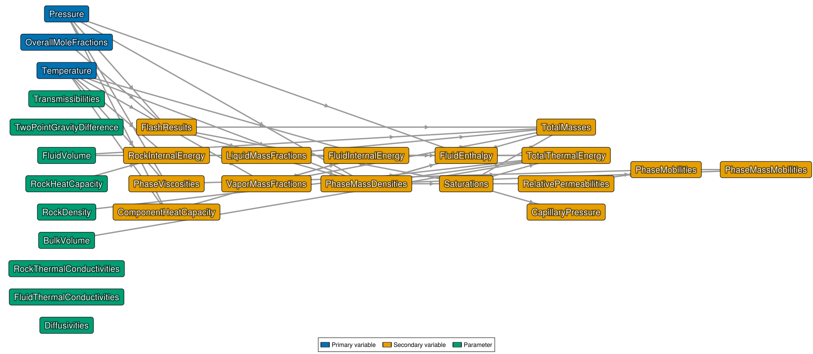
The starting point of the GPU implementation was thus a design suitable for transferring to GPUs, but that had not been tested on GPUs outside the linear solver for six years. I had performed a few conceptual tests of running the some of the heavier properties on GPUs during work on the OPM Flow GPU implementation, which essentially was application of Adapt to some large constructors. I also did a few tests on our automatic differentiation tests from Jutul.jl to confirm that it was suitable for GPUs for simple heat equation models. We can then go section for section through the required porting work:

Properties on GPUs

At the outset, properties seemed like the biggest hurdle. JutulDarcy has a large number of secondary variables that cover geothermal, compositional, blackoil, tracers and enhanced oil recovery. Let us take as example one of the CO$_2$-brine mixing density properties that implements the correlation from _Density of aqueous solutions of CO$2$ by J.E. Garcia, 2001:

 1
 2
 3
 4
 5
 6
 7
 8
 9
10
11
12
13
14
15
16
17
18
19
20
21
22
23
24
25
26
27
28
29
30
31
32
33
34

struct BrineCO2MixingDensities{T} <: AbstractCompositionalDensities
    tab::T
    coeffs::NTuple{4, Float64}
end

function BrineCO2MixingDensities(tab::T; coefficients = (37.51, −9.585e−2, 8.74e−4, −5.044e−7)) where T
    return BrineCO2MixingDensities{T}(tab, coefficients)
end

@jutul_secondary function update_density!(rho, rho_def::BrineCO2MixingDensities, model::SimulationModel{D, S}, Pressure, Temperature, LiquidMassFractions, ix) where {D, S<:CompositionalSystem}
    c1, c2, c3, c4 = rho_def.coeffs
    sys = model.system
    l, v = phase_indices(sys)
    for i in ix
        p = Pressure[i]
        T = Temperature[i]
        X_co2 = LiquidMassFractions[2, i]
        rho_h2o_pure, rho_co2 = rho_def.tab(p, T)
        rho_brine = co2_brine_mixture_density(T, c1, c2, c3, c4, rho_h2o_pure, X_co2)
        rho[v, i] = rho_co2
        rho[l, i] = rho_brine
    end
end

function co2_brine_mixture_density(T_kelvin, c1, c2, c3, c4, rho_h2o_pure, X_co2)
    T = T_kelvin - 273.15 # Relation is in C, input is in Kelvin
    vol_co2 = 1e−6*(c1 + c2*T + c3*T^2 + c4*T^3)
    rho_liquid_co2_pure = 44.01e-3/vol_co2
    X_h2o = 1.0 - X_co2
    # Linear volume mixing rule
    vol = X_co2/rho_liquid_co2_pure + X_h2o/rho_h2o_pure
    # Return as density
    return 1.0/vol
end

This is a fairly complicated function that encodes a relationship between named inputs (Pressure, Temperature, LiquidMassFractions) and the density output for a specific type of compositional models. The definition has an internal table for pure phase properties (i.e. brine without CO$_2$, CO$_2$ without vaporized water) that it evaluates. Before the brine density is written to the return array, it is corrected to account for the dissolved CO$_2$ mass fraction.

To get this running on the GPU, two changes were needed. I had to add an Adapt call to automatically generate transfers to GPU, and I had to manually adapt the interpolation type:

 1
 2
 3
 4
 5
 6
 7
 8
 9
10
11
12

# In JutulDarcy
Adapt.@adapt_structure BrineCO2MixingDensities
# In Jutul
function Adapt.adapt_structure(to, interpolant::BilinearInterpolant)
    return BilinearInterpolant(
        Adapt.adapt(to, interpolant.X),
        Adapt.adapt(to, interpolant.Y),
        Adapt.adapt(to, interpolant.F),
        Adapt.adapt(to, interpolant.lookup_x),
        Adapt.adapt(to, interpolant.lookup_y)
    )
end

That’s it! Note that there are no changes to the functions that define the mathematical model for the density. The required changes are only applied to the types and not to the functions has two important implications:

1. As there are no changes to the functional form, we do not have to force modellers to write relationships in a special manner for it to run on GPUs.
2. Verification of a GPU port is much easier when there are no changes to the functions themselves. If rewriting an expression for GPU introduces subtle changes in behavior, the simulator will still happily simulate the wrong answer, but changes to types will result in compilation errors.

Once I had a working approach for porting individual properties, I set up a small test harness and let Codex with Sol 5.6 work for a few hours fixing and testing the remaining property evaluations during the weekend while I did some carpentry around the house (at least I have a backup career if the coding agents take over completely).

Equations on GPUs

The model equations were also an exercise in using Adapt. In addition, I let Sol port one of my old codes for fuzing equation evaluation with assembly. This code was not very useful on CPU, where memory is abundant, but on GPU it saves substantial memory. Many parts of the code had to be slightly modified to handle asynchronous operations and transfer to and from GPUs during input and output, but there were no changes to the outer API or the governing equations themselves. As with the properties, this means that the verification process is limited to checking if the code compiles and runs rather than going over every single functional expression.

Convergence and updates on GPUs

These functions were straightforward to transfer to GPUs. Several fused for-loops that computed several things at once had to be cleaned up. In my opinion, adding GPU support reduced the complexity of this part of the code.

Linear solvers on GPUs

I have had the GPU implementation on my TODO-list for a long time. The largest barrier was always the linear solver, which usually amounts to a significant amount of the model runtime. JutulDarcy uses a mixture of hypre (which has Julia bindings for CPU/MPI and is hassle-free to bundle), a hand-written block ILU(0) and standard Julia sparse functions. If I wanted a vendor-neutral implementation, my options were:

1. Add support for the vendor libraries. We already support CuSPARSE and AMGX for CUDA, and similar implementations are available for AMDGPU (with the rolls-off-your-tongue name rocALUTION). However, AMGX is not actively maintained, only builds on Linux and the performance is not as good as one would hope from a native GPU solver.
2. Build support for hypre with different GPU backends, and add this support to the Julia package. This definitely the most practical option that uses pre-existing libraries and still on my TODO list. However, it is a fair bit of engineering efforts to build the different GPU variants and integrate them with the Julia binary builder system, and figuring out compilation options is definitely not my best skill.
3. Write our own AMG and preconditioner library from scratch using KernelAbstractions as the execution model.

One problem with reservoir simulation is that the linear solver does a lot of repeat work for successive solves of “almost” the same linear system, which is not well supported in the open source AMG solvers. I have written a fair number of simple AMG codes on CPU before, but I was a bit hesitant to do this myself. Existing libraries, like hypre, have been hardened over decades. However, after thinking a bit about my options, I saw that there was an opportunity to make a limited library that:

• Focused on reuse of hierarchies and memory for the repeated solves of similar linear systems with the same sparsity structure
• Was limited to scalar AMG with the most useful coarsening variants
• Works in parallell on a single node (i.e. no multi-node or multi-GPU support)

This is a quite limited subset of what most hypre supports, but it sufficiently covers the needed routines for solving flow systems.

This has been an on-and-off project for me. The first attempt can be found in the form of Draugr.jl which was intended primarily to test the capabilities of agents, as no code was written by humans in that project. The performance was quite good, but after many agent sessions the code was far too expansive to integrate directly into JutulDarcy. So I set up a test fixture with exported matrices that allowed the code to run tests against hypre and our own smoothers, wrote a specification with a proposed API and let Sol work for several sessions. The resulting library is quite small - about 4000 lines of code compared to Draugr’s 12290 lines of code. The AMG is very similar to the best performing options from hypre, to the extent that I would consider the AMG implementation as a derived work of hypre.

The nice thing about preconditioners is that it is very easy to verify their performance by checking if the application of the preconditioner $P$ gives a new update $x = P^{-1}b$ that reduces the linear residual $| Ax - b |_2$ at a reasonable speed for sample systems $A$. As the interface to the simulator is quite limited and easy to test, I am comfortable letting an agent work on this part without going over every line of code. In the future, it is likely that we can switch to builds of hypre for different devices. Jutul also has the option to use vendor libraries where preconditioners exist, but having a Julia native preconditioner means that we can automatically generalize support of JutulDarcy to any other backend that may appear in the future ³

Putting it all together

The results are a much faster solver for both forward and backward solves. This applies not only to GPU, but also to CPU, where we can now finally launch very fast threaded simulations in an interactive manner. The ergonomics of running with threads versus MPI for interactive work cannot be understated, as MPI requires manually launching a new set of processes that then produce output on disk.

The benchmark numbers indicate that a unified implementation based on automatic differentiation does not sacrifice anything in terms of fast performance on different devices. In a sense, we can have our cake and eat it too!

I finally note that the SPE10 benchmark is a classical benchmark that is often (mis-)used. The simulation scenario is very simple and most of the complexity comes from the high heterogeneity in the model. As most robust simulators can take very large time-steps in this setting, total simulation times for the case comes down to how aggressive time-stepping you make use of. Looking at the per-iteration breakdown is more illustrative as it removes the effect of time-step selection and nonlinear tolerances.

Working with agents

I have found a good rhythm with agents where I use a mixture of VSCode with the agent to do pair-programming and the dedicated application for more open-ended tasks where I want the agent to investigate autonomously and then have a look at the outcomes myself at a later stage. The changes to the main code is an example of the former where I want to inspect every line, while the preconditioners fall in the latter category.

Frontier models like Sol are very good at doing software engineering tasks, but my experience is that their efficiency more or less mirrors the code they are working against. If a task was not easy to do in the first place, they have a tendency to engineer hacks that a human would likely not bother writing. I suppose this comes from the model’s reinforcement learning that emphasizes a working solution highly. Another capability that likely comes from the same training is a greatly improved efficiency for agents to run smaller subsets of code to figure out issues and performance.

The models now quickly build minimal tests, extract pieces of code into local fixtures and make reports on performance. This makes the models much more efficient at practical scientific software engineering than at the start of 2026, even if the reasoning quality has not increased by the same magnitude. After an agent has worked for several hours, their working directory will be littered with code tests, log files and other artifacts. I suspect that even if the models stay at the same level in terms of reasoning quality, there is a lot more to be gained in how they are applied. Exciting times ahead…

Concluding remarks

Being able to run everything on GPUs is definitely a nice milestone, but I consider the real advantage of this work to be a future-proofing. The current GPU prices may make it hard to justify when you can easily pay more than a 100,000 USD for a top of the line GPU, versus a tenth of that for e.g. a Threadripper CPU. Still, running models on hardware that is both much more parallel and more restricted in terms of instruction sets seems to be the future. With KernelAbstractions as the foundation, we are ready to test whatever comes next.